Chapter 10 Selecting The Best Model
It’s always of interest to compare the results of one model to another (or even more) to determine the “best” model to share with some else. On the other hand, it’s easy to get carried away with trying out different models in an attempt to make performance improvements especially when the might only be marginally better.
It’s also wise to pick methods that you know how to reasonably defend over those that you can’t. For example, picking a Neural Net model might result in better accuracy although if you are challenged on the results in some way, would you be able to address all concerns ? If a logistic regression model resulted in a comparable result then you might should stick with that result since it’s a well-known method that few would question.
10.1 An Example
As an example, let’s go back to the linear modeling example back in the section wherein we introduced the caret package.
set.seed(123) # Make this example reproducible
idx <- createDataPartition(mtcars$mpg, p = .8,
                           list = FALSE,
                           times = 1)
head(idx)
## Resample1
## [1,] 1
## [2,] 3
## [3,] 4
## [4,] 5
## [5,] 6
## [6,] 8example_Train <- mtcars[ idx,]
example_Test <- mtcars[-idx,]
#
control <- trainControl(method = "cv", # Cross Fold
number = 5, # 5 Folds
verboseIter = FALSE) # Verbose
# Train the model
set.seed(123) # Make this example reproducible
my_lm <- train(mpg ~ wt,
example_Train,
method = "lm",
trControl = control)
my_lm## Linear Regression
##
## 28 samples
## 1 predictor
##
## No pre-processing
## Resampling: Cross-Validated (5 fold)
## Summary of sample sizes: 22, 22, 23, 22, 23
## Resampling results:
##
## RMSE Rsquared MAE
## 2.674278 0.8128595 2.255329
##
## Tuning parameter 'intercept' was held constant at a value of TRUE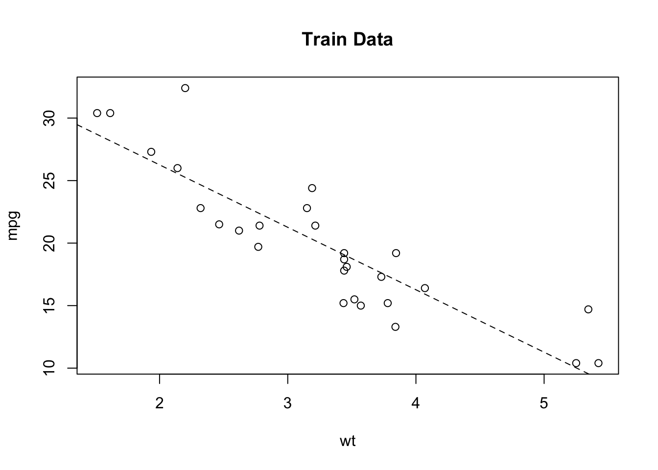
So does this model perform better than a model built using a support vector machine ? It’s easy to generate such a model by reusing much of the same information from above.
This is arguably one of the best features of the caret package as it helps us execute any number of models and then assess their performance on new data. Let’s look at our models thus far. In fact, it’s so easy to generate them with caret, we’ll just make them here again. Let’s set a common trainControl list. We’ll use the Train and Test sets from above.
#set.seed(123) # Make this example reproducible
my_svm <- train(
  mpg ~ wt,
  example_Train,
  method = "svmRadial",
  trControl = control
)

my_svm
## Support Vector Machines with Radial Basis Function Kernel
##
## 28 samples
## 1 predictor
##
## No pre-processing
## Resampling: Cross-Validated (5 fold)
## Summary of sample sizes: 23, 21, 23, 22, 23
## Resampling results across tuning parameters:
##
## C RMSE Rsquared MAE
## 0.25 3.827559 0.7700785 2.907836
## 0.50 3.127704 0.8035070 2.418092
## 1.00 2.962344 0.7735412 2.441182
##
## Tuning parameter 'sigma' was held constant at a value of 4.935503
## RMSE was used to select the optimal model using the smallest value.
## The final values used for the model were sigma = 4.935503 and C = 1.So let’s plot the training data as well as the resulting regression line (in the color black) coming from the lm object. We’ll also plot the results from the Support Vector Machine predictions on the same graph (in red). From this plot it appears that the Support Vector Machine does a better job of “following” the actual data - at least for the training data.
We might even be able to improve the SVM performance if we tune the hyperparameters but the default without tuning seems better than the lm. It’s this type of observation that leads one to consider if there are yet other methods that would result in even better results.
plot(mpg~wt,data=example_Train,main="Train Data")
abline(lm_fit$finalModel)
grid()
svm_preds <- predict(my_svm,example_Train)

pdf <- data.frame(cbind(Train$wt,svm_preds))
points(svm_preds~V1,data=pdf[order(pdf$V1),],col="red",pch=4,type="l")
legend("topright",c("lm","svm"),col=c("black","red"),lty=1,cex=1)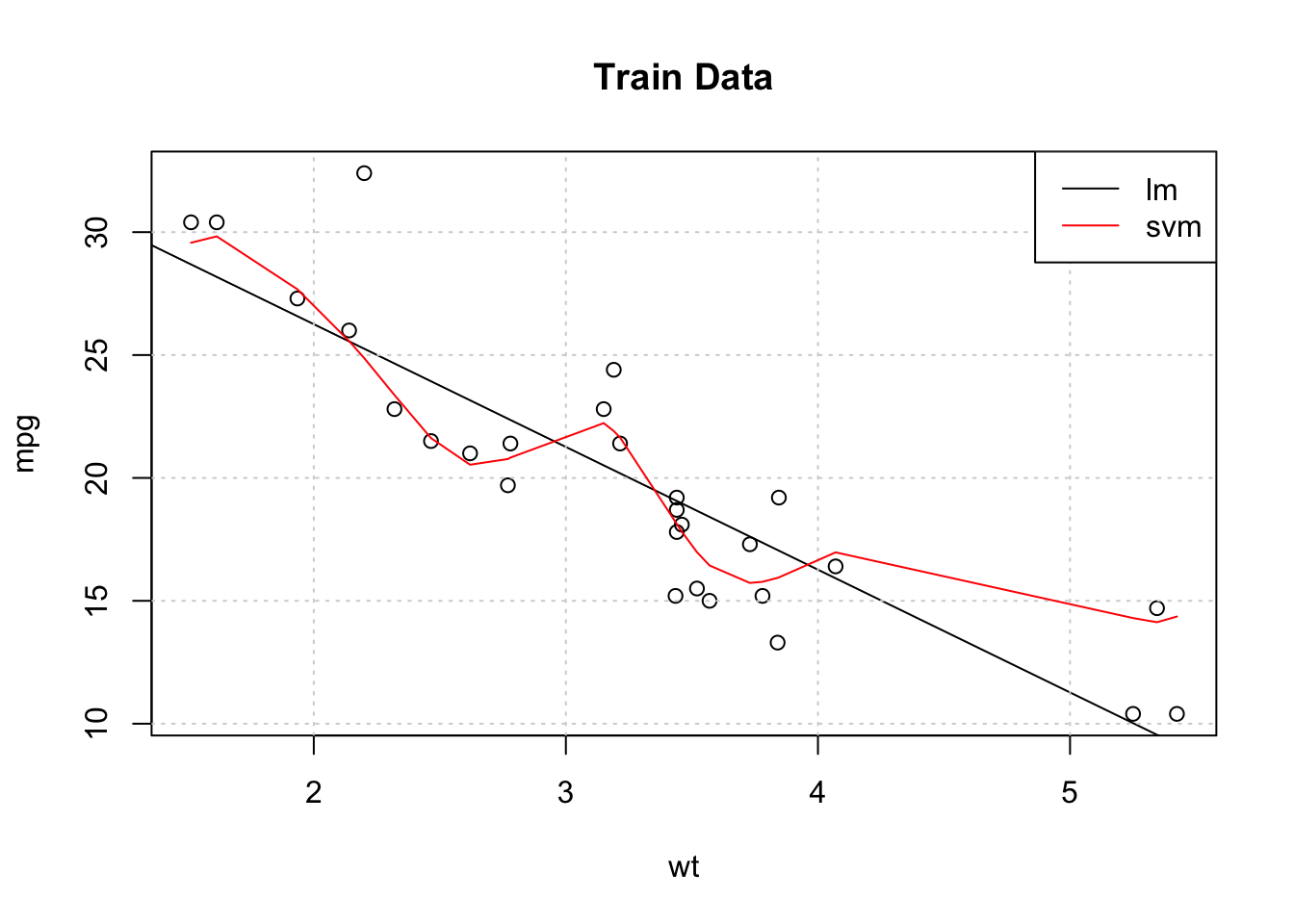
In terms of the RMSE for the Test set predictions, which method is better (i.e. the lowest RMSE) ?
lm_preds <- predict(my_lm,example_Test)
svm_preds <- predict(my_svm,example_Test)
#
cat("RMSE for lm is: ",Metrics::rmse(example_Test$mpg,lm_preds),"\n")
## RMSE for lm is: 4.622936## RMSE for svm is: 4.25258910.2 More Comparisons
Let’s keep going. We’ll use some more methods to see how they perform on the same data. The cool thing about caret is that we can reuse the same control object and seeds to facilitate reproducibility. We’ll pick two other methods in addition to the ones we have to see how we can compare them all. In reality, this would be just the beginning of the process, not the end since if we pick a method with hyperparameters then we would want to tune those.
control <- trainControl(method = "cv",       # Cross Fold
                        number = 5,          # 5 Folds
                        verboseIter = FALSE)  # Verbose
Note that we will be predicting the MPG value as a function of all variables in the data frame.
# Train the lm model
set.seed(123)
comp_mod_lm <- train(mpg ~ .,
                     example_Train,
                     method = "lm",
                     trControl = control)


# Train the SVM Radial Model
set.seed(123)
comp_mod_svm <- train(mpg ~ .,
                     example_Train,
                     method = "svmRadial",
                     trControl = control)

# Train the Lasso and Elastic-Net Regularized Generalized Linear Models
set.seed(123)
comp_mod_glmnet <- train(mpg ~ .,
                     example_Train,
                     method = "glmnet",
                     trControl = control)

# Train the Random Forest Model
set.seed(123)
comp_mod_ranger <- train(mpg ~ .,
                     example_Train,
                     method = "ranger",
                     trControl = control)
10.3 Using the resamples() function
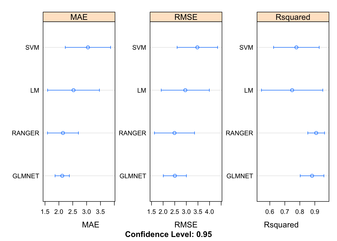
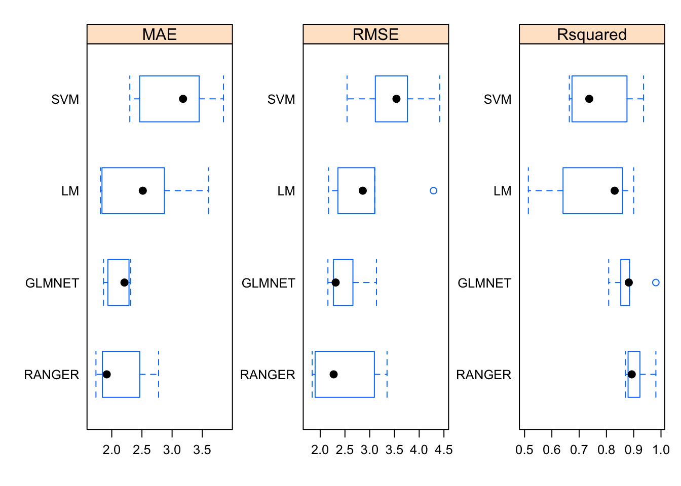
Now, here comes the “magic”. Because we built four different modeling objects on the same data set and seeds we can now use the resamples function to collect, analyze, and visualize a set of results. This is pretty powerful.
results <- resamples(list(LM     = comp_mod_lm,
                          SVM    = comp_mod_svm,
                          GLMNET = comp_mod_glmnet,
                          RANGER = comp_mod_ranger))

summary(results)
##
## Call:
## summary.resamples(object = results)
##
## Models: LM, SVM, GLMNET, RANGER
## Number of resamples: 5
##
## MAE
## Min. 1st Qu. Median Mean 3rd Qu. Max. NA's
## LM 1.812441 1.837600 2.514336 2.528231 2.871953 3.604825 0
## SVM 2.298816 2.461957 3.181394 3.048435 3.448238 3.851768 0
## GLMNET 1.862535 1.935960 2.210150 2.121240 2.285487 2.312070 0
## RANGER 1.737802 1.844707 1.916262 2.147651 2.463621 2.775865 0
##
## RMSE
## Min. 1st Qu. Median Mean 3rd Qu. Max. NA's
## LM 2.168345 2.358031 2.859978 2.955532 3.102042 4.289265 0
## SVM 2.542181 3.113981 3.540769 3.474628 3.762321 4.413890 0
## GLMNET 2.156074 2.266042 2.312372 2.506638 2.661106 3.137597 0
## RANGER 1.837313 1.897020 2.271997 2.490290 3.094805 3.350313 0
##
## Rsquared
## Min. 1st Qu. Median Mean 3rd Qu. Max. NA's
## LM 0.5138034 0.6409778 0.8302200 0.7487594 0.8588454 0.8999503 0
## SVM 0.6640028 0.6738122 0.7370650 0.7772563 0.8753710 0.9360303 0
## GLMNET 0.8083109 0.8525418 0.8819329 0.8816976 0.8845961 0.9811066 0
## RANGER 0.8695032 0.8793320 0.8928333 0.9091406 0.9228603 0.9811743 0We can visualize the results. For whatever reason, the caret package favors use of the lattice graphics package. Most of the work here is in telling the dotplot function that we need to plot each of the metrics on its own respective scale to improve viewabilty.
10.4 Model Performance
Of course, we can now use the Test data frame to see how the RMSE looks on the holdout data frame.
## [1] 4.808981## [1] 3.65783## [1] 3.768203## [1] 2.28841210.5 Feature Evaluation
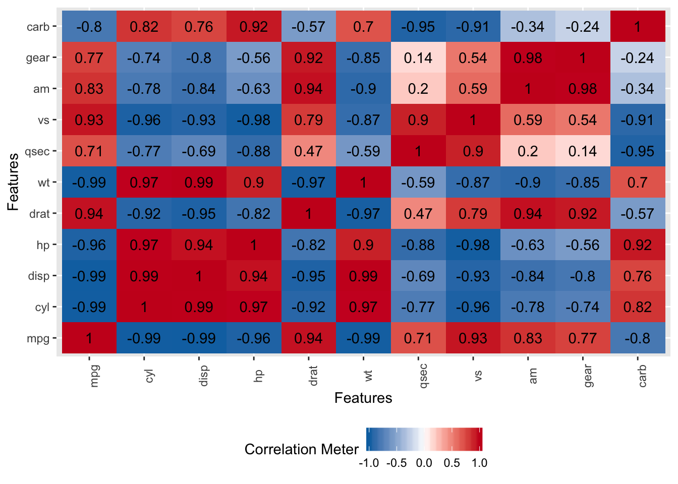
Features are the columns in your data set. Up until now we have not been concerned with the formula being specified choosing rather to focus on how to run models with the caret package. However, knowing how to select the “best” subset of features is important since an overspcified formula might result in very long training times and, even then, it might not be that good of a model for predicting out of sample error. Of course, various methods have ways to deal with this problem.
For example, Stepwise regression is one way to look at combinations of predictor variables to arrive at the optimal feature set according to some score (e.g. AIC, BIC). This process is implemented recursively. However, none of this should be a substitute for solid intuition about the data or knowing how features vary with each other (if at all). Still, packages such as caret have ways to assist with feature selection.
A benefit of using something like Random Forests is that as part of its output it can inform us what variables it considers to be important. In reality it has to do this since it does publish information like R Squared values, coefficients or p-values.
##        %IncMSE
## cyl  12.182582
## disp 13.516104
## hp   12.846467
## drat  4.705008
## wt   12.682193
## qsec  3.941303
## vs    2.913989
## am    2.895120
## gear  3.145579
## carb  4.863950
This gives us some clues as to what variables we might want to include or exclude in our formula.
10.5.1 Identifying Redundant Features
Lots of Data Scientists and model builders would like to know which features are important and which are redundant - BEFORE building the model. Many times, people just include all features and rely upon post model statistics to diagnose the model. This is fine though there are automated methods to help. Some statisticians do not like this approach (e.g. Step Wise Regression) because it emphasizes a scoring metric that is computed as a function of other measures though that process itself might be incomplete in some way. Ideally, you would have some up front idea about the data.
10.5.3 Ranking Features
Another approach would be to identify the important variables as determined by a rigorous, reliable and statistically aware process. Some models will report this information as part of the computation. The caret package has a function called varImp which helps to calculate relative variable importance within an object produced by the train function. What this means for us is that we can take most models built with train and pass it to the varImp function.
set.seed(123)
idx <- createDataPartition(mtcars$mpg, p = .8,
                                  list = FALSE,
                                  times = 1)
train <- mtcars[ idx,]
test  <- mtcars[-idx,]

myLm <- train(mpg~.,
                     data = train,
                     method = "lm",
                     metric = "RMSE")
## Warning in predict.lm(modelFit, newdata): prediction from a rank-deficient fit
## may be misleading## Linear Regression
##
## 28 samples
## 10 predictors
##
## No pre-processing
## Resampling: Bootstrapped (25 reps)
## Summary of sample sizes: 28, 28, 28, 28, 28, 28, ...
## Resampling results:
##
## RMSE Rsquared MAE
## 4.851577 0.6068996 3.870965
##
## Tuning parameter 'intercept' was held constant at a value of TRUE##
## Call:
## lm(formula = .outcome ~ ., data = dat)
##
## Residuals:
## Min 1Q Median 3Q Max
## -3.2742 -1.3609 -0.2707 1.1921 4.9877
##
## Coefficients:
## Estimate Std. Error t value Pr(>|t|)
## (Intercept) -2.81069 22.93545 -0.123 0.904
## cyl 0.75593 1.21576 0.622 0.542
## disp 0.01172 0.01674 0.700 0.494
## hp -0.01386 0.02197 -0.631 0.536
## drat 2.24007 1.77251 1.264 0.223
## wt -2.73273 1.87954 -1.454 0.164
## qsec 0.53957 0.71812 0.751 0.463
## vs 1.21640 2.02623 0.600 0.556
## am 1.73662 2.08358 0.833 0.416
## gear 2.95127 1.88459 1.566 0.136
## carb -1.19910 0.98232 -1.221 0.239
##
## Residual standard error: 2.431 on 17 degrees of freedom
## Multiple R-squared: 0.8861, Adjusted R-squared: 0.8191
## F-statistic: 13.23 on 10 and 17 DF, p-value: 3.719e-06If you look at the summary of the model it looks pretty bleak because most of the coefficients aren’t significant. You wouldn’t want to take your career on this model.
Now let’s see what variables are considered to be important by using varImp. Remember that this might lead us to use a subset of the more prominent variables in the formation of a new model in case, for example, the coefficients in the existing model weren’t significant.
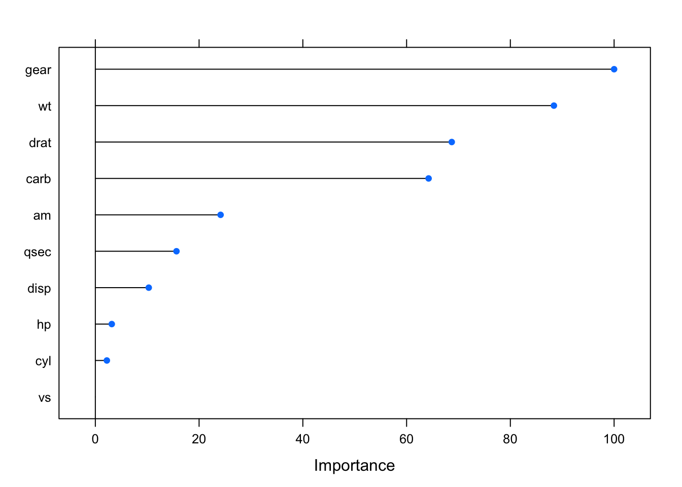
How do things look in the model if we limit the formula to some of the “important” (allegedly) features ? Well, it explains more of the variance with fewer predictors (the R^2 value). Both wt and hp are significant. That’s a start.
## Linear Regression
##
## 28 samples
##  3 predictor
##
## No pre-processing
## Resampling: Bootstrapped (25 reps)
## Summary of sample sizes: 28, 28, 28, 28, 28, 28, ...
## Resampling results:
##
##   RMSE      Rsquared   MAE
##   2.432624  0.8324283  1.903699
##
## Tuning parameter 'intercept' was held constant at a value of TRUE##
## Call:
## lm(formula = .outcome ~ ., data = dat)
##
## Residuals:
## Min 1Q Median 3Q Max
## -4.2197 -1.4116 -0.0793 0.7964 5.8604
##
## Coefficients:
## Estimate Std. Error t value Pr(>|t|)
## (Intercept) 21.8969 6.3475 3.450 0.002086 **
## wt -3.2324 0.7559 -4.276 0.000262 ***
## drat 3.0962 1.2957 2.390 0.025075 *
## carb -0.8783 0.3277 -2.680 0.013093 *
## ---
## Signif. codes: 0 '***' 0.001 '**' 0.01 '*' 0.05 '.' 0.1 ' ' 1
##
## Residual standard error: 2.414 on 24 degrees of freedom
## Multiple R-squared: 0.8414, Adjusted R-squared: 0.8216
## F-statistic: 42.45 on 3 and 24 DF, p-value: 9.421e-1010.5.4 Feature Selection
Being able to automatically include only the most important features is desirable (again an example might be Step Wise Regression). Caret provides its own function to do a simple backwards selection to recursively eliminate features based on how they contribute (or not) to the model. You could do all of this by hand yourself of course.
Automatic feature selection methods can be used to build many models with different subsets of a dataset and identify those attributes that are and are not required to build an accurate model. The caret package has a function called *rfe** to implement this. However, it involves some additional setup:
rfeControl <- rfeControl(functions=lmFuncs, method="cv", number=5)

set.seed(123)
results <- rfe(x = train[,2:11],
               y = train[,1],
               sizes=c(2:11),
               rfeControl=rfeControl)

print(results)
##
## Recursive feature selection
##
## Outer resampling method: Cross-Validated (5 fold)
##
## Resampling performance over subset size:
##
## Variables RMSE Rsquared MAE RMSESD RsquaredSD MAESD Selected
## 2 3.372 0.6377 2.814 0.9630 0.2797 0.8355
## 3 3.344 0.6551 2.676 1.0886 0.3338 0.9744
## 4 2.447 0.7540 2.092 0.6355 0.3001 0.5221
## 5 2.413 0.7835 2.103 0.8479 0.2216 0.6835
## 6 2.466 0.8024 2.113 0.6500 0.2013 0.4734
## 7 2.341 0.7905 1.934 0.6261 0.2318 0.5776 *
## 8 2.379 0.7761 1.978 0.6606 0.2648 0.5698
## 9 3.015 0.7153 2.474 0.8629 0.2616 0.6155
## 10 3.171 0.7163 2.605 0.8324 0.2551 0.5222
##
## The top 5 variables (out of 7):
## gear, wt, drat, am, vs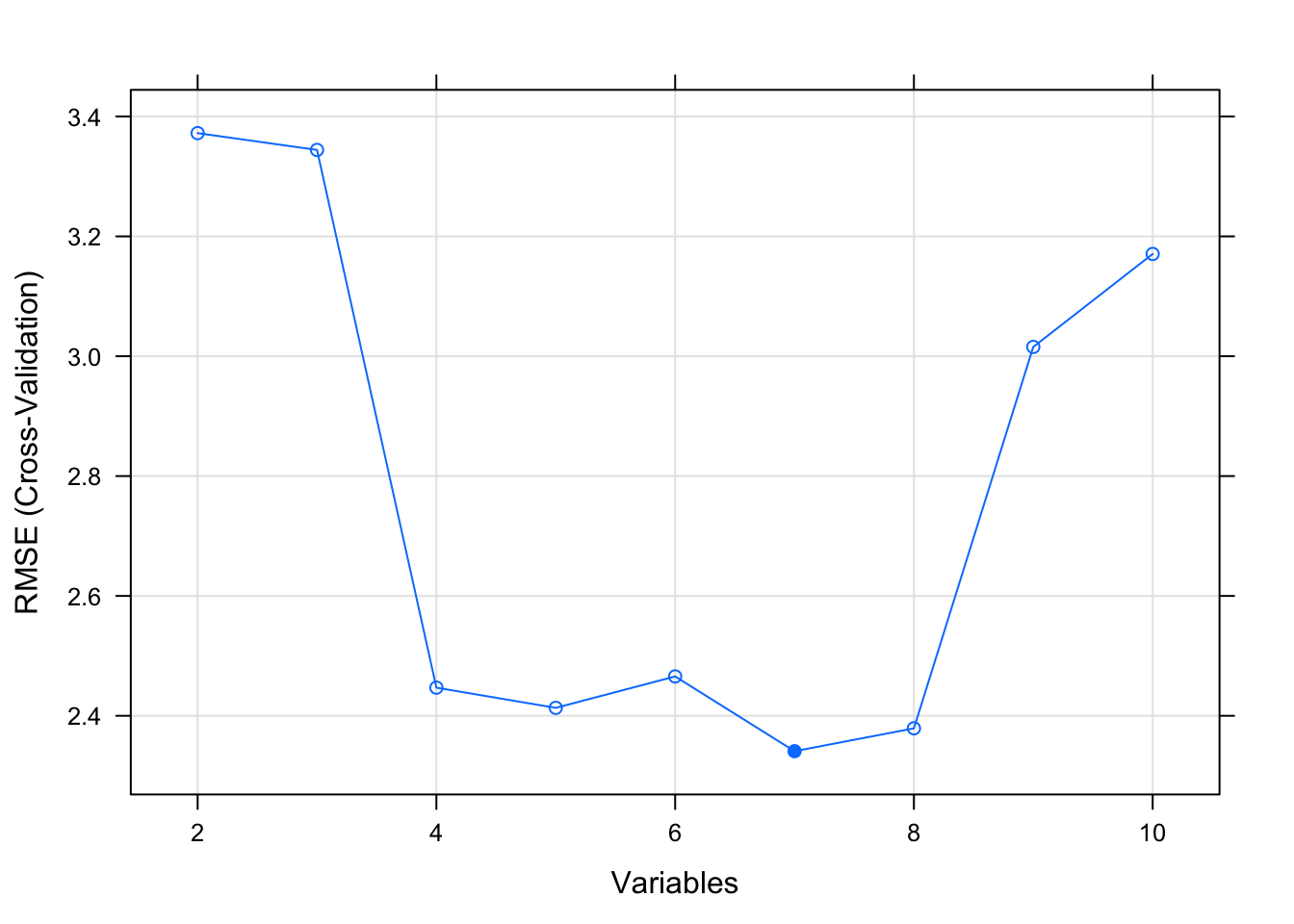
## Linear Regression
##
## 28 samples
##  3 predictor
##
## No pre-processing
## Resampling: Bootstrapped (25 reps)
## Summary of sample sizes: 28, 28, 28, 28, 28, 28, ...
## Resampling results:
##
##   RMSE      Rsquared   MAE
##   3.392751  0.6848952  2.708587
##
## Tuning parameter 'intercept' was held constant at a value of TRUE##
## Call:
## lm(formula = .outcome ~ ., data = dat)
##
## Residuals:
## Min 1Q Median 3Q Max
## -4.7657 -1.8714 0.1848 1.0130 6.8310
##
## Coefficients:
## Estimate Std. Error t value Pr(>|t|)
## (Intercept) 27.5335 7.1808 3.834 0.0008 ***
## wt -4.3232 0.7679 -5.630 8.52e-06 ***
## drat 2.1989 1.5420 1.426 0.1667
## gear -0.3563 1.0098 -0.353 0.7273
## ---
## Signif. codes: 0 '***' 0.001 '**' 0.01 '*' 0.05 '.' 0.1 ' ' 1
##
## Residual standard error: 2.744 on 24 degrees of freedom
## Multiple R-squared: 0.795, Adjusted R-squared: 0.7694
## F-statistic: 31.03 on 3 and 24 DF, p-value: 1.997e-0810.5.5 Recursive Feature Elimination
The general idea with this approach is to build models using combinations of predictors to arrive at the best model according to some metric such as RMSE. Some predictors might be discarded along the way resulting in a “leaner” feature set that would then hopefully be easier to defend than a more complex or fully specified feature set.
There is no free lunch here in that blindly accepting the features handed to you by a recursive or automatic method should not be considered authoritative especially if you have a reason to believe that some key feature has been excluded. Many people, however, like to use these methods as a starting point. You would still need to review the diagnostics associated with a final model to determine if it is statistically sound.
According to the caret documentation there are a large number of supported models that contain some form of embedded or built-in feature selection. Such functions are doing you a favor (or not) by showing you the importance of contributing features.
10.5.5.1 An Example
Let’s work with the lm function again to see if we can find some interesting features using some caret functions. The main function for Recursive Feature Elimination is rfe which, like the train function, accepts a control object to help guide the process. Here we are telling the rfe function to use some helper functions to assess predictors. We don’t need to pass it a model - it handles these things under the hood. In this case we’ll use 10 Fold Cross Validation.
set.seed(123)
control <- rfeControl(functions=lmFuncs, method="cv",number=10)

results <- rfe(mtcars[,2:11],     # Predictor features
               mtcars[,1],        # Predicted features - mpg
               sizes=c(1:5),      # pick groups of predictors 1-5
               rfeControl=control)
results
##
## Recursive feature selection
##
## Outer resampling method: Cross-Validated (10 fold)
##
## Resampling performance over subset size:
##
## Variables RMSE Rsquared MAE RMSESD RsquaredSD MAESD Selected
## 1 3.113 0.8486 2.762 1.878 0.2403 1.811
## 2 3.134 0.8392 2.798 1.650 0.2689 1.568
## 3 2.700 0.8872 2.421 1.366 0.1543 1.203 *
## 4 2.916 0.8655 2.512 1.444 0.1664 1.239
## 5 2.992 0.8884 2.633 1.438 0.1461 1.253
## 10 3.391 0.8864 3.055 1.447 0.1614 1.283
##
## The top 3 variables (out of 3):
## wt, am, drat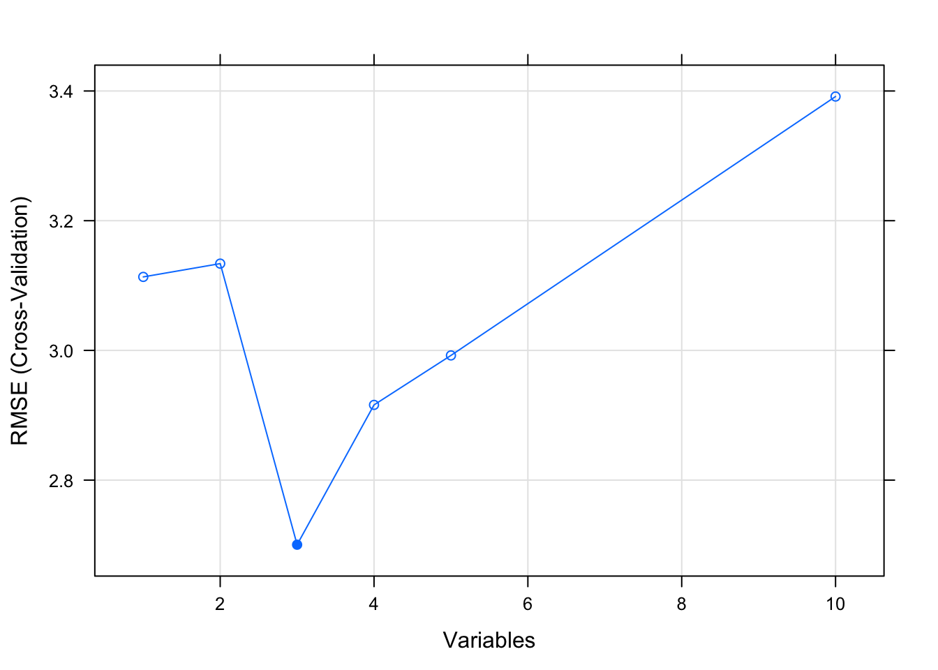
What we get back is some idea about the important features. We could then build a model with caret that uses only these features to see if the suggested RMSE value mentioned in the rfe process matches.
