Chapter 2 Getting Hands On
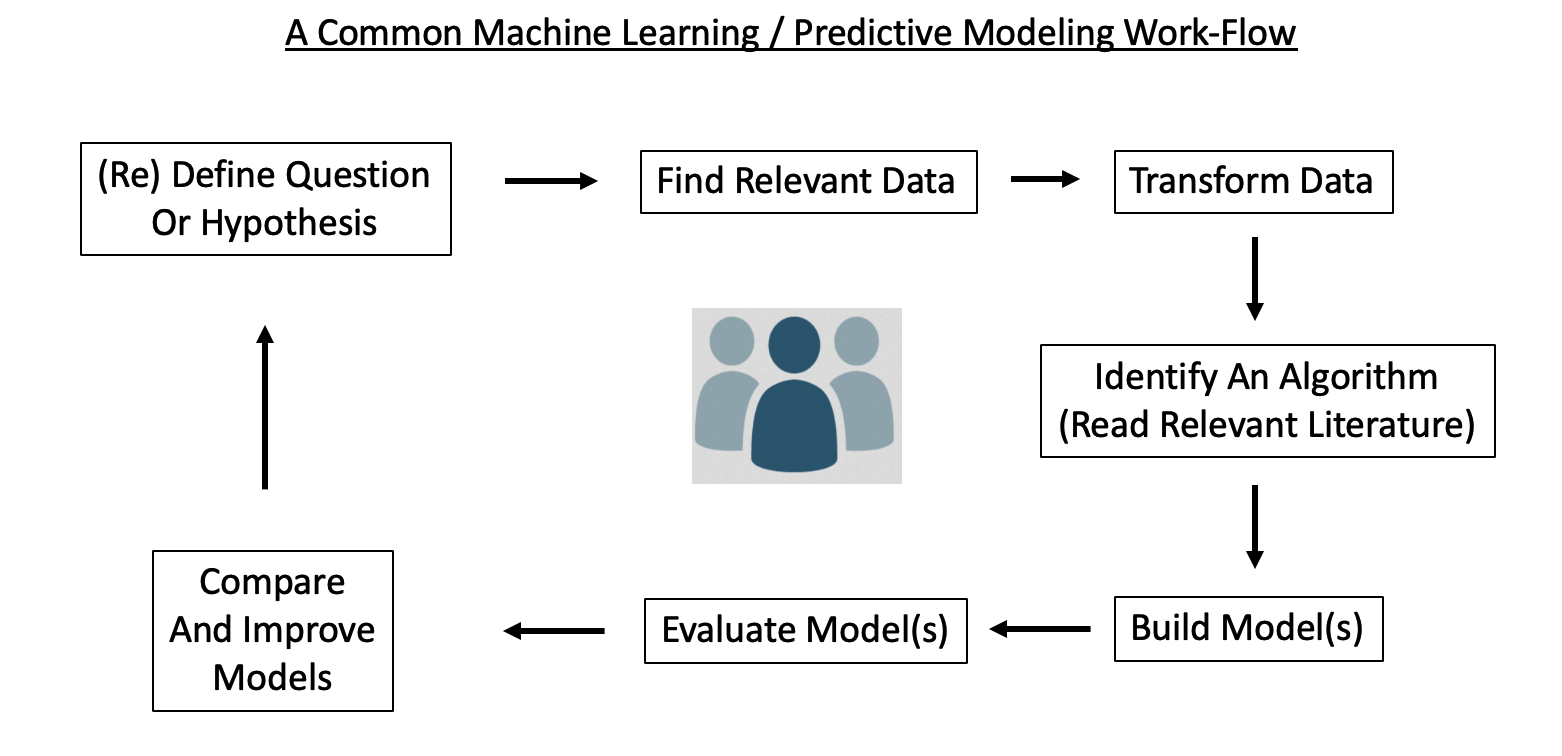
Here is a high level over view of an ML work flow. Note that:
- It is a cycle, quite likely to be repeated multiple times before arriving at some actionable result
- The driving questions / hypotheses are subject to change, redefinition, or abandonment
- Multiple people might be involved
To get the ball rolling with a practical case, let’s consider the Pima Indians Data Frame. Read in a copy.
url <- "https://raw.githubusercontent.com/steviep42/bios534_spring_2020/master/data/pima.csv"
pm <- read.csv(url)

head(pm)
## pregnant glucose pressure triceps insulin mass pedigree age diabetes
## 1 6 148 72 35 0 33.6 0.627 50 pos
## 2 1 85 66 29 0 26.6 0.351 31 neg
## 3 8 183 64 0 0 23.3 0.672 32 pos
## 4 1 89 66 23 94 28.1 0.167 21 neg
## 5 0 137 40 35 168 43.1 2.288 33 pos
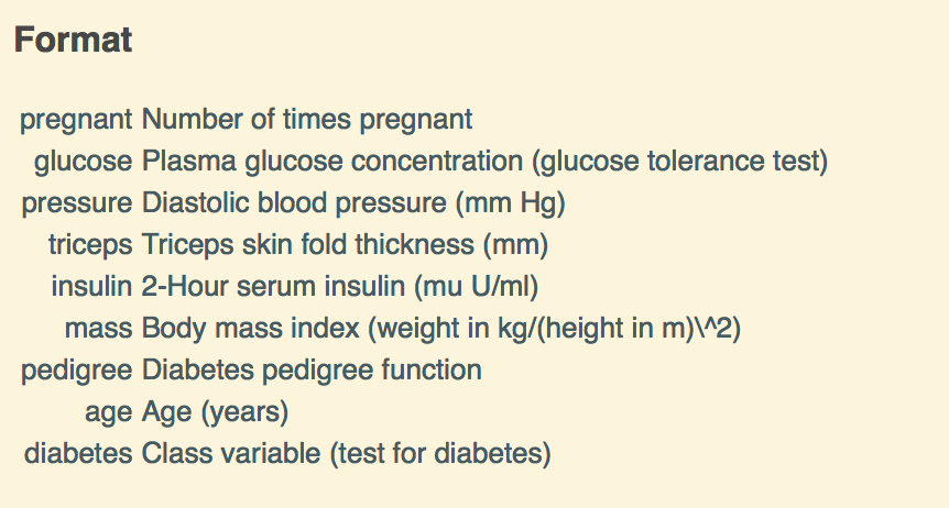
## 6 5 116 74 0 0 25.6 0.201 30 negThe description of the data set is as follows:
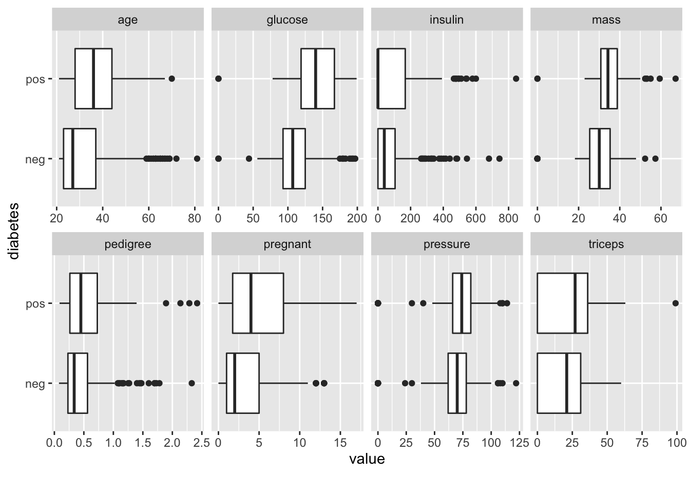
So we now have some data on which we can build a model. Our defining question or driving motivation might be how to predict whether someone will be postitive for diabetes based on other variables within the data. Is glucose, for example, an important variable to consider ?
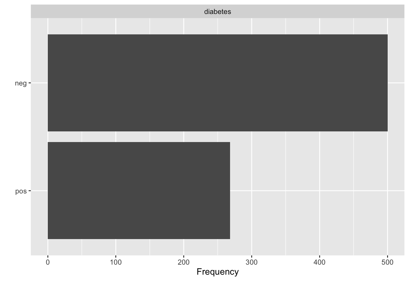
In lookin at the data, there is a variable in the data called “diabetes” which indicates the disease / diabetes status (“pos” or “neg”) of the person. It would be good to come up with a model that we could use with incoming data to determine if someone has diabetes.
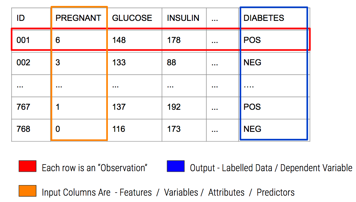
2.1 Important Terminology
In predictive modeling there are some common terms to consider:
2.2 Exploratory Plots
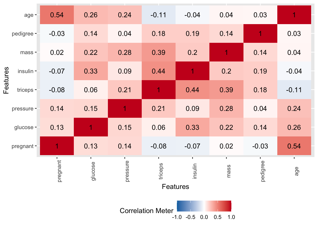
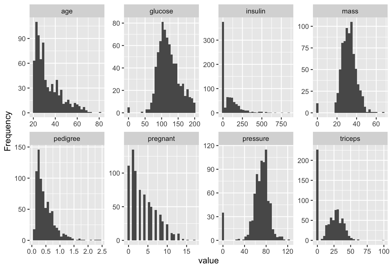
We’ll look use some stock plots from the DataExplorer package to get a feel for the data. Look at correlations between the variables to see if any are strongly correlated with the variable we wish to predict or any other variables.