Chapter 2 XML and JSON
This is where things get a little dicey because some web pages will return XML and JSON in response to inquiries and while these formats seem complicated they are actually doing you a really big favor by doing this since these formats can ususally be easily parsed using various packges. XML is a bit hard to get your head around and JSON is the new kid on the block which is easier to use.
Since this isn’t a full-on course lecture I’ll keep it short as to how and why you would want to use these but any time you spend trying to better understand JSON (and XML) the better of you will be when parsing web pages. It’s not such a big deal if all you are going to be parsing is raw text since the mthods we use to do that avoid XML and JSON although cleaning up raw text has its own problems. Let’s revisit the Wikipedia example from the previous section.
library(rvest)

# Use read_html to fetch the webpage
url <- "https://en.wikipedia.org/wiki/World_population"
ten_most_df <- read_html(url)

ten_most_populous <- ten_most_df %>%
  html_nodes("table") %>% `[[`(5) %>% html_table()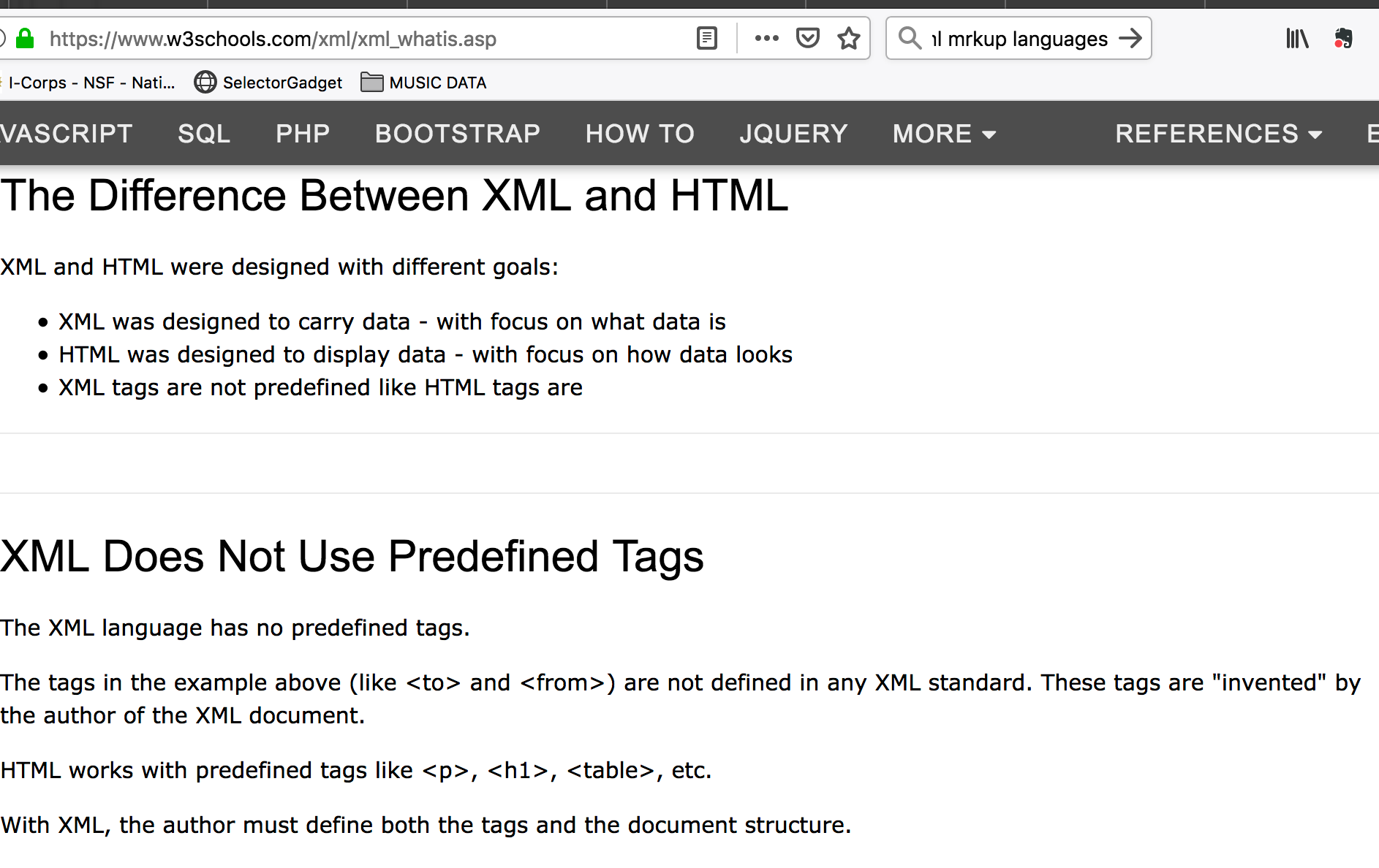
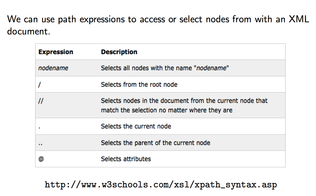
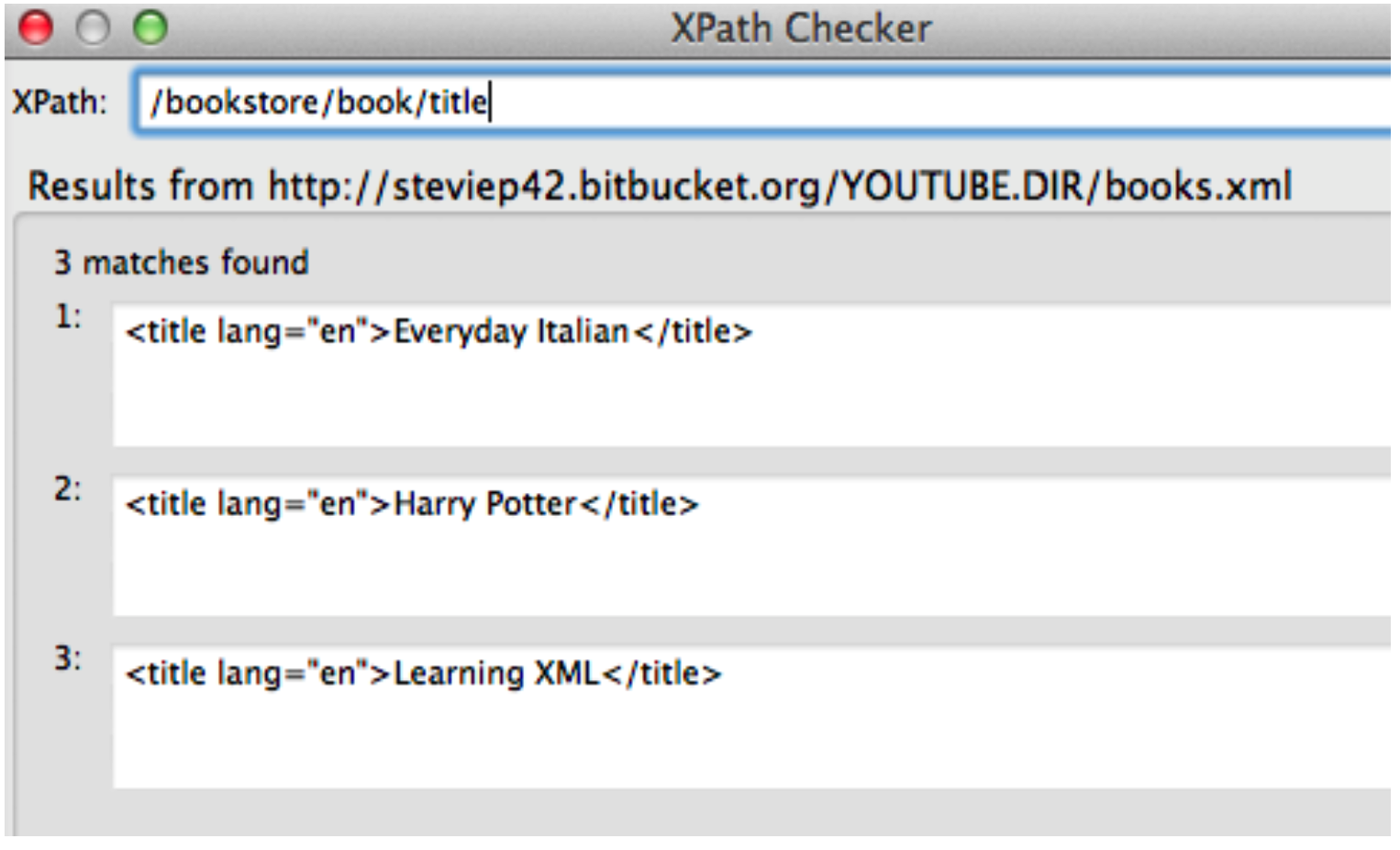
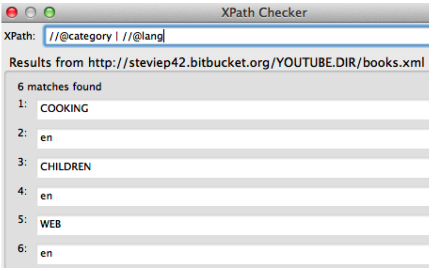
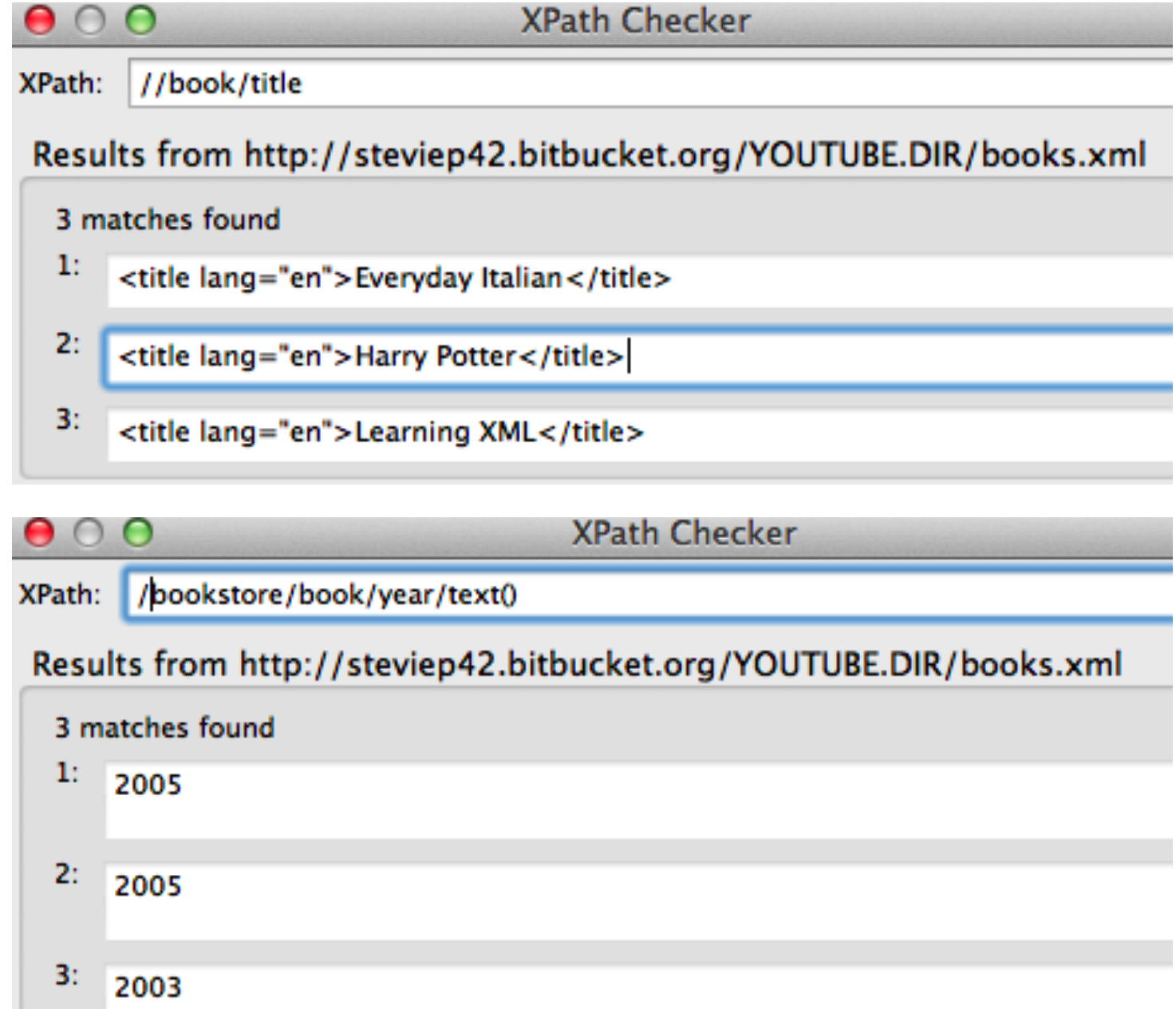
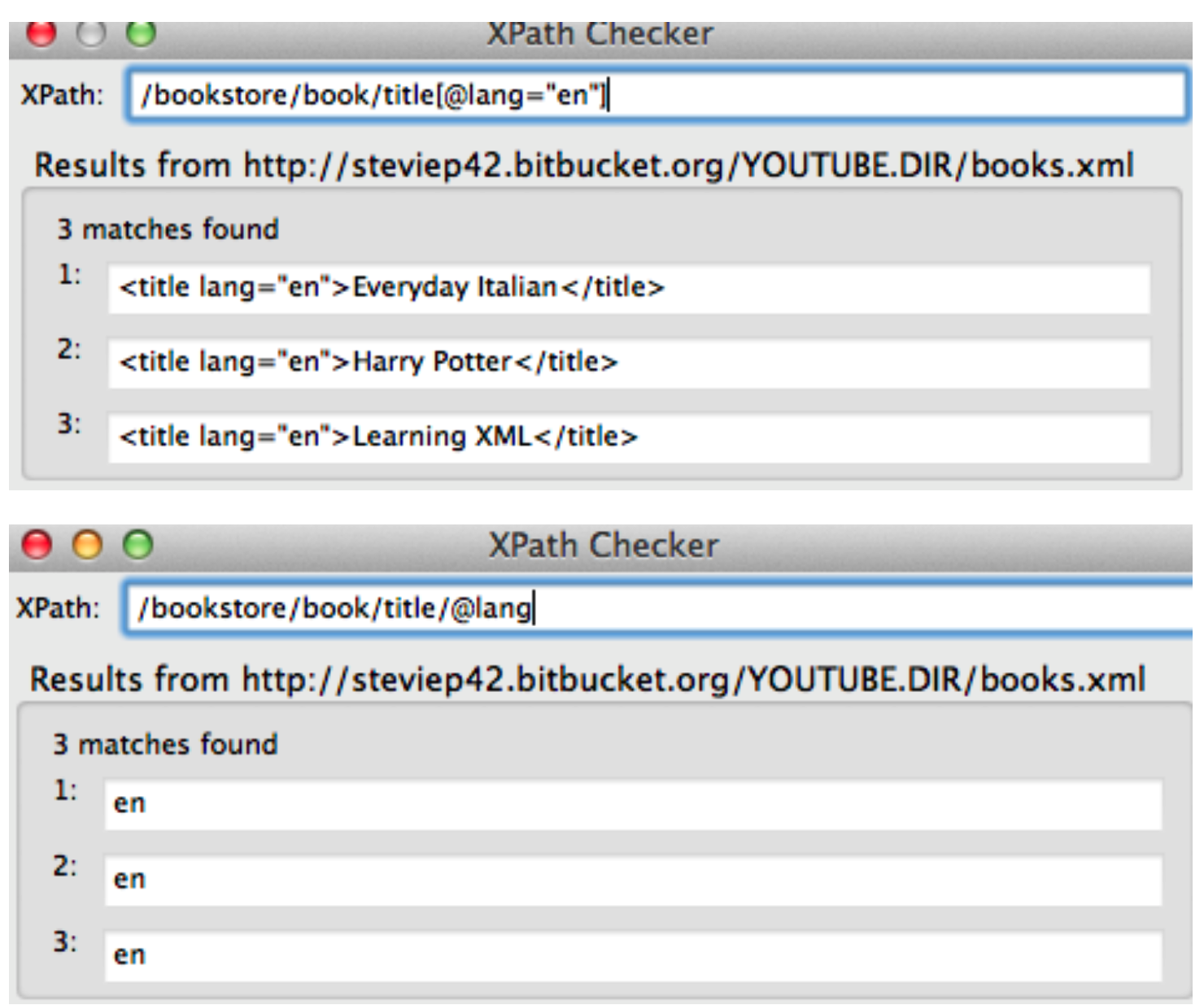
Let’s look at an XML file that has some basic content:
<?xml version="1.0" encoding="UTF-8"?>
<bookstore>
<book category="COOKING">
<title lang="en">Everyday Italian</title>
<author>Giada De Laurentiis</author>
<year>2005</year>
<price>30.00</price>
</book>
<book category="CHILDREN">
<title lang="en">Harry Potter</title>
<author>J K. Rowling</author>
<year>2005</year>
<price>29.99</price>
</book>
<book category="WEB">
<title lang="en">Learning XML</title>
<author>Erik T. Ray</author>
<year>2003</year>
<price>39.95</price>
</book>
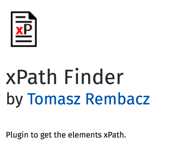
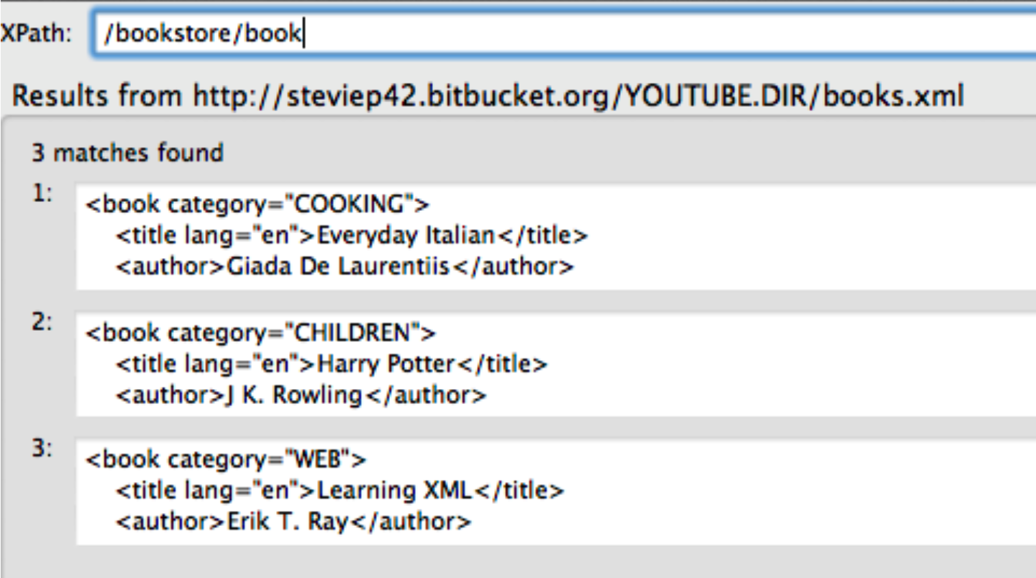
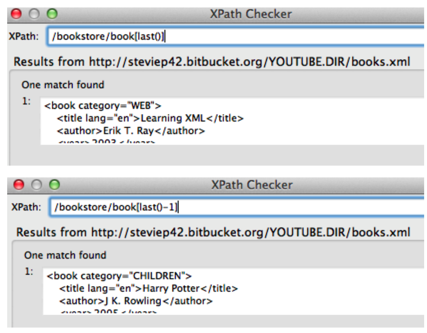
</bookstore>Well we pulled out all tables and then, by experimentation, we isolated table 6 and got the content corresponding to that. But. Is there a more direct way to find the content ? There is. It requires us to install some helper plugins such as the xPath Finder for Firefox and Chrome. In reality there are a number of ways to find the XML Path or CSS Path for an element within a web page but this is a good one to start.
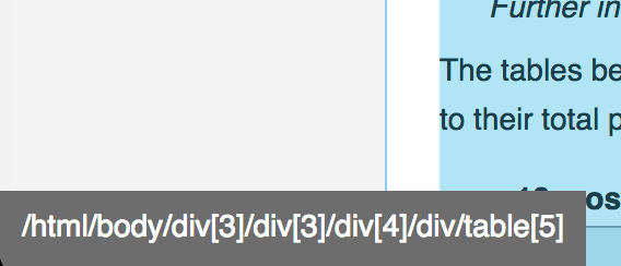
Remeber that we want to find the table corresponding to the “10 Most Populous Countries.” So we activate the xPath finder plugin and the highlight the element of interest. This takes some practice to get it right. Once you highlight the desired elment you will see the corresponding XPATH. Here is a screenshot of what I did. We can use the resulting path to directly access the table without first having to first pull out all tables and then trying to find the right one
# Use read_html to fetch the webpage
url <- "https://en.wikipedia.org/wiki/World_population"
ten_most_populous <- read_html(url)

ten_most_df <- ten_most_populous %>%
  html_nodes(xpath='/html/body/div[3]/div[3]/div[5]/div[1]/table[4]') %>%
  html_table()

# We have to get the first element of the list.
ten_most_df <- ten_most_df[[1]]

ten_most_df
## # A tibble: 10 × 6
## Rank Country Population `% of world` Date `Source(official or UN)`
## <int> <chr> <chr> <chr> <chr> <chr>
## 1 1 China 1,411,860,200 17.8% 8 Feb 2022 National population clock[90]
## 2 2 India 1,387,792,351 17.5% 8 Feb 2022 National population clock[91]
## 3 3 United States 333,191,720 4.20% 8 Feb 2022 National population clock[92]
## 4 4 Indonesia 269,603,400 3.40% 1 Jul 2020 National annual projection[93]
## 5 5 Pakistan 220,892,331 2.79% 1 Jul 2020 UN Projection[94]
## 6 6 Brazil 214,324,314 2.70% 8 Feb 2022 National population clock[95]
## 7 7 Nigeria 206,139,587 2.60% 1 Jul 2020 UN Projection[94]
## 8 8 Bangladesh 172,180,722 2.17% 8 Feb 2022 National population clock[96]
## 9 9 Russia 146,748,590 1.85% 1 Jan 2020 National annual estimate[97]
## 10 10 Mexico 127,792,286 1.61% 1 Jul 2020 National annual projection[98]2.1 Finding XPaths
In addition to Browser Plugins there are standalone tools such as the Oxygen XML Editor which is availabel through the Emory Software Express Website. This is a comprehensive XML editor that will allow you to parse XML and develop paths to locate specific nodes within an XML document. If you find yourself working with websites with lots of XML then this will be useful. The Oxygen editor is free.
Let’s look at an XML file that has some basic content:
<?xml version="1.0" encoding="UTF-8"?>
<bookstore>
  <book category="COOKING">
    <title lang="en">Everyday Italian</title>
    <author>Giada De Laurentiis</author>
    <year>2005</year>
    <price>30.00</price>
  </book>
  <book category="CHILDREN">
    <title lang="en">Harry Potter</title>
    <author>J K. Rowling</author>
    <year>2005</year>
    <price>29.99</price>
  </book>
  <book category="WEB">
    <title lang="en">Learning XML</title>
    <author>Erik T. Ray</author>
    <year>2003</year>
    <price>39.95</price>
  </book>
</bookstore>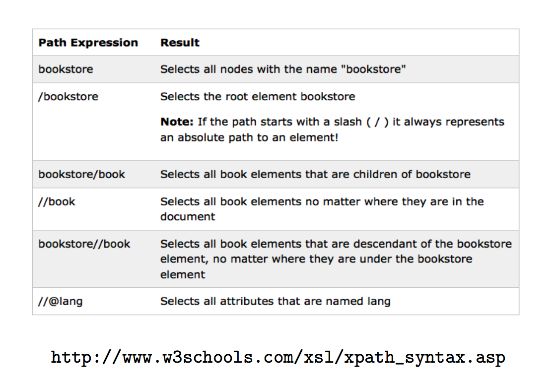
2.2 Example: GeoCoding With Google
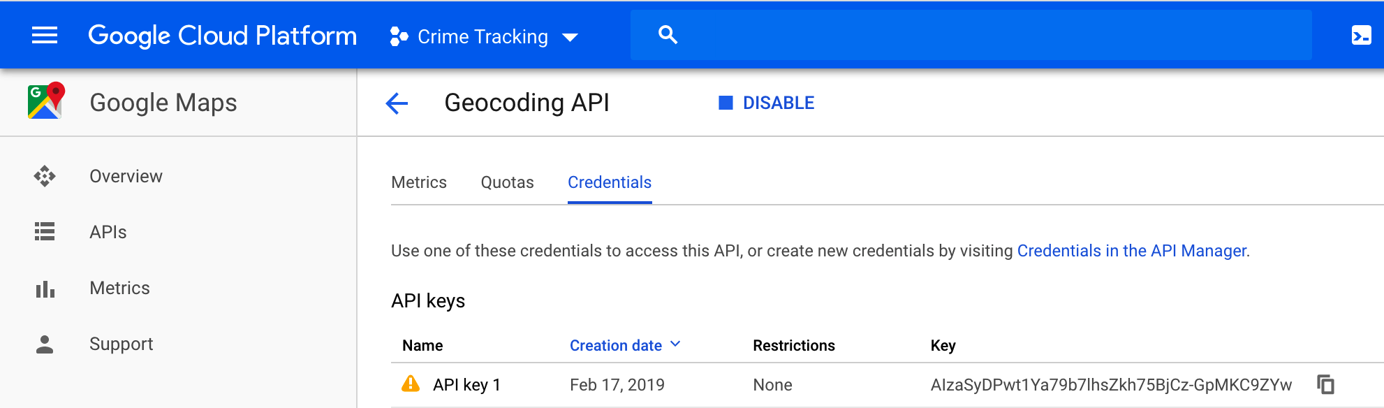
Let’s run through an example of using the GeoCoding API with Google. They used to provide free access to this service but no more. You have to sign up for an account and get an API key. If you are currently taking one of my classes I probably have arranged for cloud credits that you can use to do Google Geocoding for free.
So one way to do this is to create a URL according to the specification given in the Google Geocoding documentation. We need 1) the base Google URL for the Geocoding service, 2) the format of the desired output (XML or JSON), 3) and address for which we want to find the latitude and longitude, and 4) the API key we create at the Google API service. Here is a fully functional URL you can paste into your browser:
If you paste this into Chome then you get something back like this:
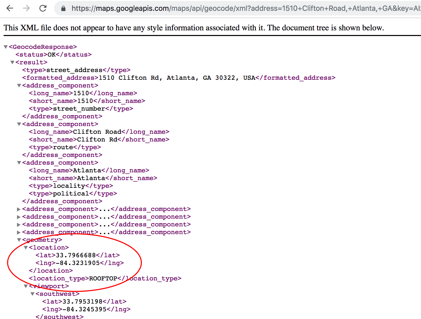
So I could create an R function to take care of this kind of thing so I could maybe pass in arbitrary addressess to be geocided. Let’s run through this example and then look at how I parsed the XML file that is returned by the Google GeoCoding API. We will stick with the 1510 Clifton Rd, Atlanta, GA address which corresponds to the Rollins Research Building.
First we will see an example of what Google returns in terms of XML. We can use some tools like Oxygen Editor (available free via Emory Software Express) to develop an appropriate XPATH expression to parse out the latitude and longitude information.
# https://maps.googleapis.com/maps/api/geocode/xml?address=1510+Clifton+Road,+Atlanta,+GA&key=AIzaSyDPwt1Ya79b7lhsZkh75BjCz-GpMKC9ZYw

# https://maps.googleapis.com/maps/api/geocode/json?address=1510+Clifton+Road,+Atlanta,+GA&key=AIzaSyDPwt1Ya79b7lhsZkh75BjCz-GpMKC9ZYw

myGeo <- function(address="1510 Clifton Rd Atlanta GA",form="xml") {
  library(XML)
  library(RCurl)

  geourl <- "https://maps.googleapis.com/maps/api/geocode/"

  # You will need to replace this with your OWN key !
  key <- "AIzaSyA3ereIVEjA0gPrxLupPLOKFGH_v98KpMA"

  address <- gsub(" ","+",address)

  add <- paste0(geourl,form,sep="?address=")
  add <- paste0(add,address,"&key=")
  geourl <- paste0(add,key)

  locale <- getURL(geourl)
  plocal <- xmlParse(locale,useInternalNodes=TRUE)

  # Okay let's extract the lat and lon
  latlon <- getNodeSet(plocal,"/GeocodeResponse/result/geometry/location/descendant::*")
  lat  <- as.numeric(xmlSApply(latlon,xmlValue))[1]
  lon  <- as.numeric(xmlSApply(latlon,xmlValue))[2]

  return(c(lat=lat,lng=lon))
}
mylocs <- myGeo()
lat lng
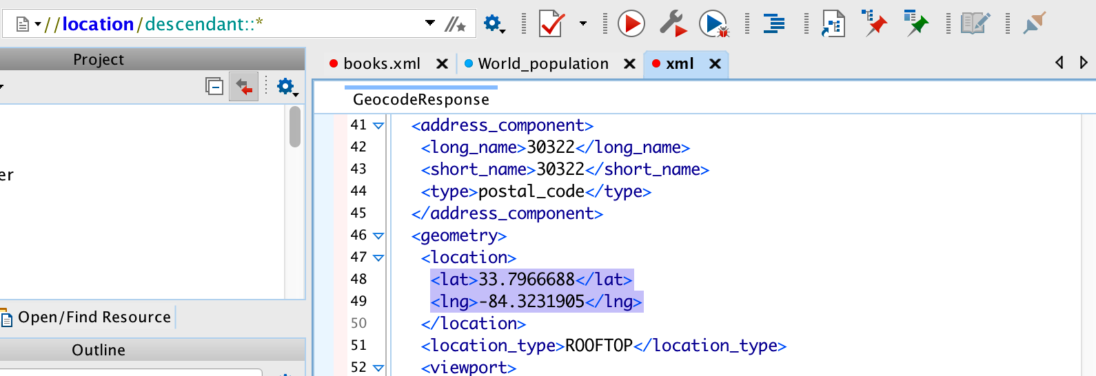
33.79667 -84.32319 Now. We could have saved the report to a file on our local computer and open it up with Oxygen editor and figure out what the approproate XPATH would be. This is basically what I did. Here is a screenshot of the session. I picked an XPATH expression of //location/descendant::*
We could expand this considerable to process a number of addresses. This is a great example of how once you get a single example working then you can generalize this into a function that will allow you to do the same thing for a much larger numnber of addressess.
namevec <- c("Atlanta GA",
             "Birmingham AL",
             "Seattle WA",
             "Sacramento CA",
             "Denver CO",
             "LosAngeles CA",
             "Rochester NY")

cityList <- lapply(namevec,myGeo,eval=FALSE)

# Or to get a data frame

cities <- data.frame(city=namevec,do.call(rbind,cityList),
stringsAsFactors = FALSE)cities## city lat lng
## 1 Atlanta GA 33.74900 -84.38798
## 2 Birmingham AL 33.51859 -86.81036
## 3 Seattle WA 47.60621 -122.33207
## 4 Sacramento CA 38.58157 -121.49440
## 5 Denver CO 39.73924 -104.99025
## 6 LosAngeles CA 34.05223 -118.24368
## 7 Rochester NY 43.15658 -77.60885# Let's create a Map
library(leaflet)
m <- leaflet(data=cities)
m <- addTiles(m)
m <- addMarkers(m,popup=cities$city)## Assuming "lng" and "lat" are longitude and latitude, respectively# Put up the Map - click on the markers
m2.3 Using JSON
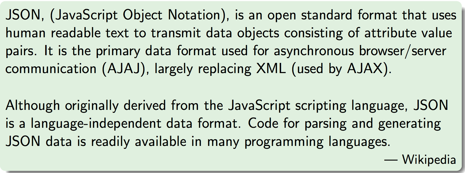
JSON is fast becoming the primary interchange format over XML although XML is still well supported. R has a number of packages to ease the parsing of JSON/ documents returned by web pages. Ususally you get back a list which is a native data type in R that can easily be manipulated into a data frame. Most web APIs provide an option for JSON or XML although some only provide JSON.
There are rules and regulations about how JSON is formed and we will learn them by example but you can look at the numerous tutotorials on the web to locate definitive references. See http://www.w3schools.com/json/ Here is an XML file that describes some employees.
<employees>
     <employee>
         <firstName>John</firstName>
         <lastName>Doe</lastName>
     </employee>
     <employee>
         <firstName>Anna</firstName>
         <lastName>Smith</lastName>
     </employee>
     <employee>
         <firstName>Peter</firstName>
         <lastName>Jones</lastName>
     </employee>
 </employees>
And here is the corresposning JSON file:
{
  "employees":[
    {"firstName":"John", "lastName":"Doe"},
    {"firstName":"Anna", "lastName":"Smith"},
    {"firstName":"Peter","lastName":"Jones"}
] }
It is important to note that the actual information in the document, things like city name, county name, latitude, and longitude are the same as they would be in the comparable XML document.
JSON documents are at the heart of the NoSQL“database”called MongoDB
JSON can be found within many webpages since it is closely related to JavaScript which is a language strongly related to web pages.
JSON is very compact and lighweight which has made it a natural followon to XML so much so that it appears to be replacing XML
See http:..www.json.org/ for a full description of the specification
An object is an unordered set of name/value pairs. An object begins with (left brace) and ends with (right brace). Each name is followed by : (colon) and the name/value pairs are separated by , (comma).
An array is an ordered collection of values. An array begins with [ (left bracket) and ends with ] (right bracket). Values are separated by , (comma).
A value can be a string in double quotes, or a number, or true or false or null, or an object or an array. These structures can be nested.
A string is a sequence of zero or more Unicode characters, wrapped in double quotes, using backslash escapes. A character is represented as a single character string.
Do you remember the Google Geocoding example from before ? We can tell Google to send us back JSON instead of XML just by adjusting the URL accordingly:
url <- "https://maps.googleapis.com/maps/api/geocode/json?address=1510+Clifton+Rd+Atlanta+GA&key=AIzaSyD0zIyn2ijIqb7OKYTGnAnchXY7zt3VB9Y"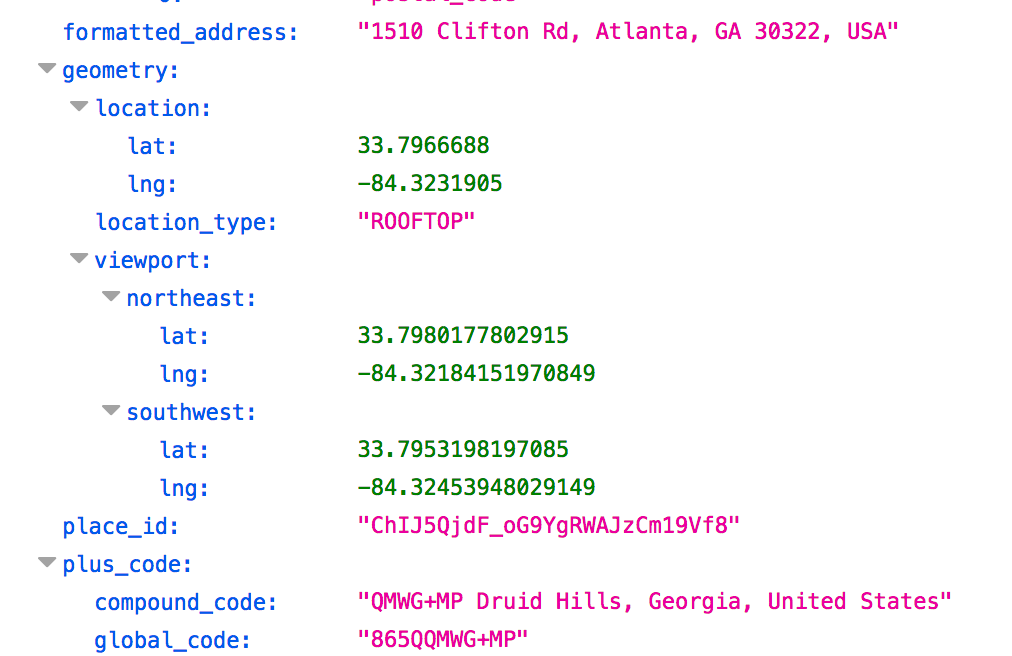
2.4 Using the RJSONIO Package
To read/parse this in R we use a package called RJSONIO. There are other packages but this is the one we will be using. Download and install it.
There is a function called fromJSON which will parse the JSON file and return a list to contain the data.
So we parse lists instead of using XPath. Many people feel this to be easier than trying to construct XPath statments. You will have to decide for yourself.
library(RJSONIO)

url <- "https://maps.googleapis.com/maps/api/geocode/json?address=1510+Clifton+Road,+Atlanta,+GA&key=AIzaSyD0zIyn2ijIqb7OKYTGnAnchXY7zt3VB9Y"
geo <- fromJSON(url)
Since what we get back is a list we can directly access whatever we want. We just index into the list. No need for complicated XPATHS.
str(geo,3)## List of 2
## $ results:List of 1
## ..$ :List of 6
## .. ..$ address_components:List of 7
## .. ..$ formatted_address : chr "1510 Clifton Rd, Atlanta, GA 30322, USA"
## .. ..$ geometry :List of 3
## .. ..$ place_id : chr "ChIJ5QjdF_oG9YgRWAJzCm19Vf8"
## .. ..$ plus_code : Named chr [1:2] "QMWG+MP Druid Hills, Georgia, United States" "865QQMWG+MP"
## .. .. ..- attr(*, "names")= chr [1:2] "compound_code" "global_code"
## .. ..$ types : chr "street_address"
## $ status : chr "OK"geo$results[[1]]$geometry$location## lat lng
## 33.79667 -84.32319Let’s put this into a function that helps us get the information for a number of addresses
myGeo <- function(address="1510 Clifton Rd Atlanta GA",form="json") {
  library(RJSONIO)

  geourl <- "https://maps.googleapis.com/maps/api/geocode/"

  # You will need to replace this with your OWN key !
  key <- "AIzaSyA3ereIVEjA0gPrxLiopLKJRPOLH_v89DpMA"

  address <- gsub(" ","+",address)

  add <- paste0(geourl,form,sep="?address=")
  add <- paste0(add,address,"&key=")
  geourl <- paste0(add,key)

  geo <- fromJSON(geourl)


  lat  <- geo$results[[1]]$geometry$location[1]
  lng  <- geo$results[[1]]$geometry$location[2]

  return(c(lat,lng))
}
Consider the following:
namevec <- c("Atlanta GA",
             "Birmingham AL",
             "Seattle WA",
             "Sacramento CA",
             "Denver CO",
             "LosAngeles CA",
             "Rochester NY")

cityList <- lapply(namevec,myGeo)

# Or to get a data frame

cities <- data.frame(city=namevec,do.call(rbind,cityList),
                     stringsAsFactors = FALSE)
Now we can check out the geocoding cities and then make a map
cities## city lat lng
## 1 Atlanta GA 33.74900 -84.38798
## 2 Birmingham AL 33.51859 -86.81036
## 3 Seattle WA 47.60621 -122.33207
## 4 Sacramento CA 38.58157 -121.49440
## 5 Denver CO 39.73924 -104.99025
## 6 LosAngeles CA 34.05223 -118.24368
## 7 Rochester NY 43.15658 -77.60885# Let's create a Map
library(leaflet)
m <- leaflet(data=cities)
m <- addTiles(m)
m <- addMarkers(m,popup=cities$city)## Assuming "lng" and "lat" are longitude and latitude, respectively# Put up the Map - click on the markers
m